39 multiple data labels excel pie chart

How to Combine or Group Pie Charts in Microsoft Excel Click on the first chart and then hold the Ctrl key as you click on each of the other charts to select them all. Click Format > Group > Group. All pie charts are now combined as one figure. They will move and resize as one image. Choose Different Charts to View your Data How to group (two-level) axis labels in a chart in Excel? This first method will guide you to change the layout of source data before creating the column chart in Excel. And you can do as follows: 1. Move the fruit column before Date column with cutting the fruit column and then pasting before the date column. 2. Select the fruit column except the column heading.

How to fix wrapped data labels in a pie chart | Sage ... 3. The data labels resize to fit all the text on one line. 4. Alternatively, by double-clicking a data label, the handles can be used to resize the label to wrap words as desired. This can be done on all data labels or on an individual slice data label. It also ensures that the labels are correctly displayed on the chart.

Multiple data labels excel pie chart

Multiple Data Labels on a Pie Chart | MrExcel Message Board So I have a table with 8 rows and 3 columns. This table includes: Column 1 - shipment name Column 2 - shipment cost Column 3 - shipment weight I have created a pie chart from this table, which covers the first two columns. Displayed next to each slice is a label with the shipment name, shipment cost, and percent share of the pie. Edit titles or data labels in a chart - support.microsoft.com The first click selects the data labels for the whole data series, and the second click selects the individual data label. Right-click the data label, and then click Format Data Label or Format Data Labels. Click Label Options if it's not selected, and then select the Reset Label Text check box. Top of Page Pie Chart in Excel | How to Create Pie Chart | Step-by ... Pie Chart in Excel is used for showing the completion or main contribution of different segments out of 100%. It is like each value represents the portion of the Slice from the total complete Pie. For Example, we have 4 values A, B, C and D.

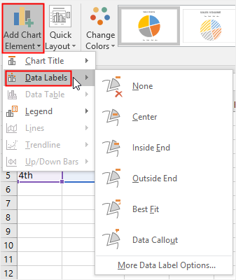
Multiple data labels excel pie chart. Create a multi-level category chart in Excel - ExtendOffice Create a multi-level category chart in Excel A multi-level category chart can display both the main category and subcategory labels at the same time. When you have values for items that belong to different categories and want to distinguish the values between categories visually, this chart can do you a favor. Multiple data labels (in separate locations on chart) Re: Multiple data labels (in separate locations on chart) You can do it in a single chart. Create the chart so it has 2 columns of data. At first only the 1 column of data will be displayed. Move that series to the secondary axis. You can now apply different data labels to each series. Attached Files 819208.xlsx‎ (13.8 KB, 263 views) Download How to add or move data labels in Excel chart? In Excel 2013 or 2016. 1. Click the chart to show the Chart Elements button . 2. Then click the Chart Elements, and check Data Labels, then you can click the arrow to choose an option about the data labels in the sub menu. See screenshot: In Excel 2010 or 2007. 1. click on the chart to show the Layout tab in the Chart Tools group. See ... Adding data labels to a pie chart - Excel General - OzGrid ... But it didn't record anything about labels, much less making them bold. In fact, I tried recording multiple macros (create the chart from scratch, modify a created chart, etc.) and still nothing about labels. The macros I recorded without touching the labels look the same as the ones with. Do you know why that is? Thanks a lot.

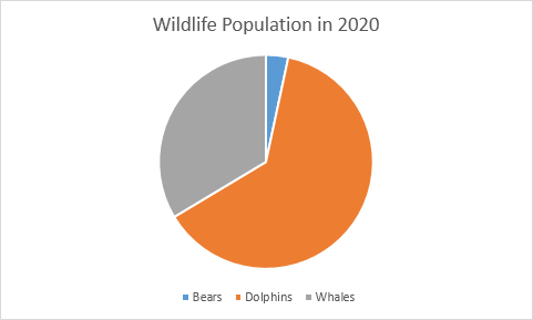
How to Create Multi-Category Charts in Excel ... Step 1: Insert the data into the cells in Excel. Now select all the data by dragging and then go to "Insert" and select "Insert Column or Bar Chart". A pop-down menu having 2-D and 3-D bars will occur and select "vertical bar" from it. Select the cell -> Insert -> Chart Groups -> 2-D Column Bar Chart Insertion Multi-Category Chart › how-to-show-percentage-inHow to Show Percentage in Pie Chart in Excel? - GeeksforGeeks Jun 29, 2021 · Select a 2-D pie chart from the drop-down. A pie chart will be built. Select -> Insert -> Doughnut or Pie Chart -> 2-D Pie. Initially, the pie chart will not have any data labels in it. To add data labels, select the chart and then click on the “+” button in the top right corner of the pie chart and check the Data Labels button. Adding second set of data labels - Excel Help Forum Excel 2007 : Adding multiple Data Labels. By ERE in forum Excel General Replies: 0 Last Post: 09-01-2010, 02:55 PM. Adding more data labels to pie chart. By ctolson in forum Excel Charting & Pivots Replies: 2 Last Post: 06-25-2010, 10:21 AM. adding extra data labels. By bagullo in forum Excel Charting & Pivots ... › doughnut-chart-in-excelHow to Create Doughnut Excel Chart? - WallStreetMojo Things to Remember About Doughnut Chart in Excel. PIE can takes only one set of data; it cannot accept more than one data series. Limit your categories to 5 to 8. Too much is too bad for your chart. Easy to compare one season’s performance against another or one to many comparisons in a single chart.

› pie-chart-examplesPie Chart Examples | Types of Pie Charts in Excel ... - EDUCBA PIE Chart can be defined as a circular chart with multiple divisions in it, and each division represents some portion of a total circle or total value. Simply each circle represents the total value of 100 per cent, and each division contributes some per cent to the total. Excel Pie Chart Multiple Labels How to Combine or Group Pie Charts in Microsoft Excel Details: Click on the first chart and then hold the Ctrl key as you click on each of the other charts to select them all. Click Format > Group > Group. All pie charts are now combined as one figure. They will move and resize as one image. Change the format of data labels in a chart To get there, after adding your data labels, select the data label to format, and then click Chart Elements > Data Labels > More Options. To go to the appropriate area, click one of the four icons ( Fill & Line, Effects, Size & Properties ( Layout & Properties in Outlook or Word), or Label Options) shown here. Solved: Show multiple data lables on a chart - Power BI 09-07-2017 06:25 AM Is there a way to display multiple labels on a chart? For example, I'd like to include both the total and the percent on pie chart. Or instead of having a separate legend include the series name along with the % in a pie chart. I know they can be viewed as tool tips, but this is not sufficient for my needs.

How to Make a Pie Chart in Excel | EdrawMax Online

A Step-By-Step Guide on How to Make a Pie Chart in Excel ... 3. Select your data values and create the chart. Highlight the data range by clicking on the cell on the top left corner and dragging it until you've selected all the cells with values you wish to include in the pie chart. Then go to the top left corner of your window and click the "Insert" tab next to the "Home" tab.

32 How To Add Y Axis Label In Excel - Labels Database 2020

How to Create Pie Charts in Excel (In Easy Steps) 6. Create the pie chart (repeat steps 2-3). 7. Click the legend at the bottom and press Delete. 8. Select the pie chart. 9. Click the + button on the right side of the chart and click the check box next to Data Labels. 10. Click the paintbrush icon on the right side of the chart and change the color scheme of the pie chart. Result: 11.

Microsoft Excel Tutorials: Add Data Labels to a Pie Chart

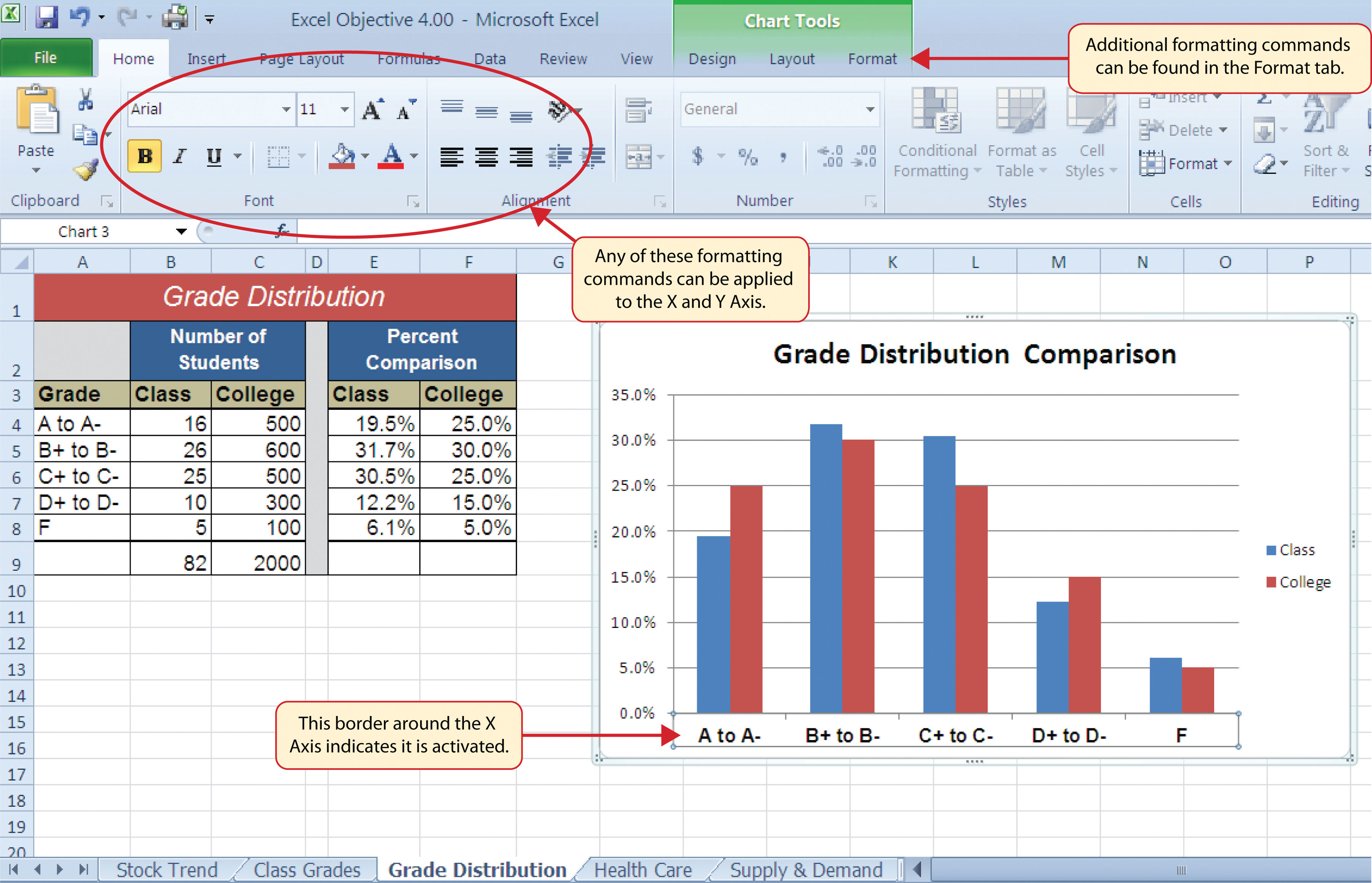
› comparison-chart-in-excelComparison Chart in Excel | Adding Multiple Series Under Same ... This window helps you modify the chart as it allows you to add the series (Y-Values) as well as Category labels (X-Axis) to configure the chart as per your need. Under Legend Entries ( S eries) inside the Select Data Source window, you need to select the sales values for the year 2018 and year 2019.

Office: Display Data Labels in a Pie Chart

Multi Level Data Labels in Charts - Beat Excel! Data: Result: A better approach is to format modify your data make multiple levels of labels before generating your chart. This way your chart will look much more professional. You don't need to make anything else. After modifying your data, just select all data as you did before and insert your chart. Excel will automatically recognize your ...