42 add data labels to pivot chart

How to add Data label in Stacked column chart of Pivot charts I'm tring to make a Pivot chart with stacked column graph. In where, i couldn't add data label for cumulative sum of value in Data label. Where i could only add data label to individual stacks in column graph. It found possible with normal stacked column chart without pivot chart. Data label in the graph not showing percentage option. only value ... Data label in the graph not showing percentage option. only value coming. Normally when you put a data label onto a graph, it gives you the option to insert values as numbers or percentages. In the current graph, which I am developing, the percentage option not showing. Enclosed is the screenshot.

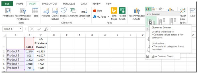
How to Create a Pivot Table: Step-by-Step - CareerFoundry All you need to do is go to the "Insert" tab in the ribbon again and select "Recommended Charts" while you are in the worksheet where your pivot table is located. Since you have already grouped the data into a pivot table, Excel starts making suggestions as to what chart will best suit your needs.

Add data labels to pivot chart

How to Add Axis Titles in a Microsoft Excel Chart Click the Add Chart Element drop-down arrow and move your cursor to Axis Titles. In the pop-out menu, select "Primary Horizontal," "Primary Vertical," or both. If you're using Excel on Windows, you can also use the Chart Elements icon on the right of the chart. Check the box for Axis Titles, click the arrow to the right, then check ... Adding a count to pivot table - Microsoft Tech Community So if family storytime happened 4 times in January and 2 times in February I would have context for the difference in attendance numbers. I am new to Pivot tables but can't seem to find a way to see this information. I do know I can click on any value and see what data was used to get that but I was hoping for something all in one table. Thanks! Excel Pivot Table Report Filter Tips and Tricks To use a pivot table field as a Report Filter, follow these steps. In the PivotTable Field list, click on the field that you want to use as a Report Filter. Drag the field into the Filters box, as shown in the screen shot below. On the worksheet, Excel adds the selected field to the top of the pivot table, with the item (All) showing.

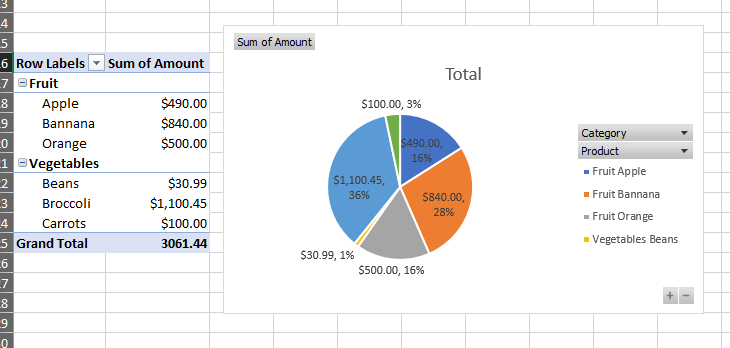
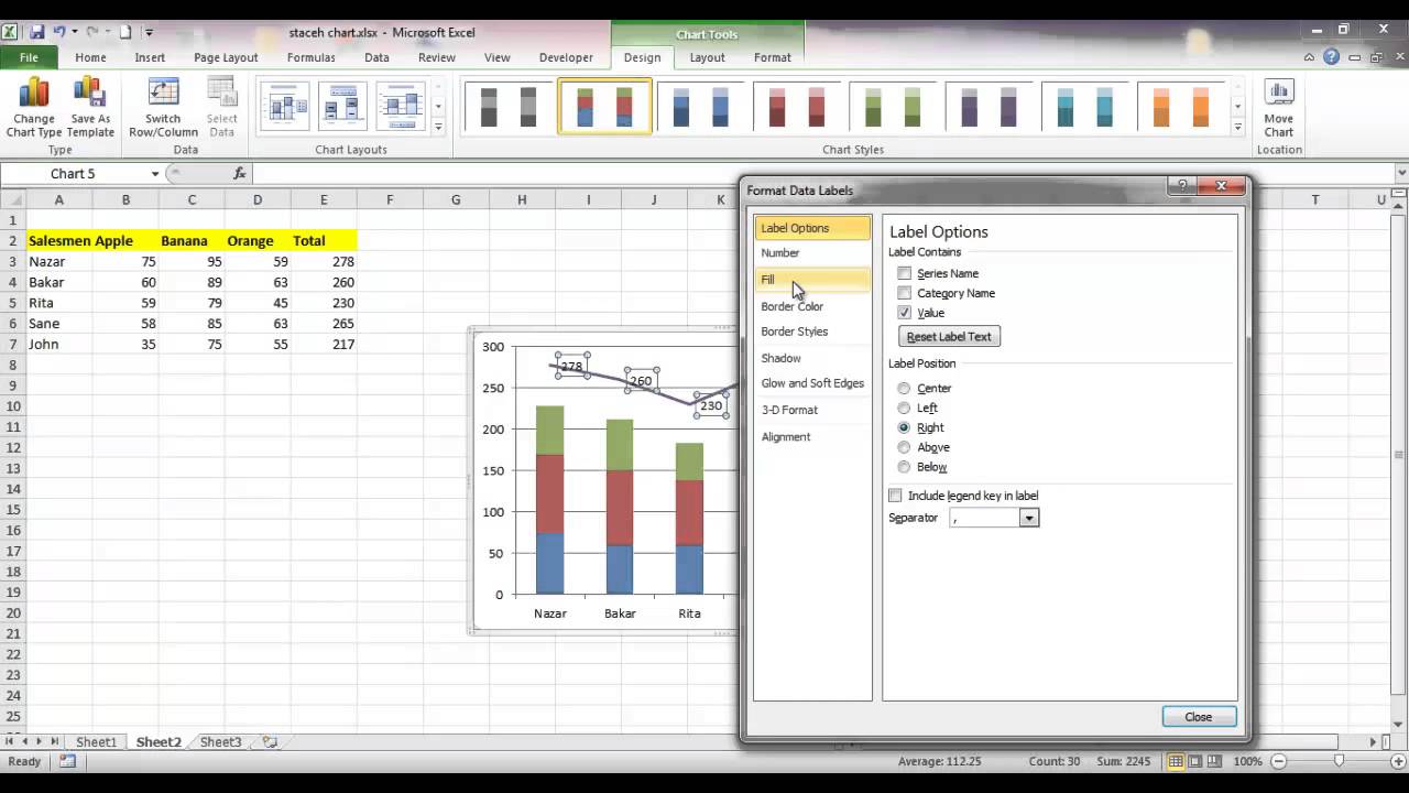
Add data labels to pivot chart. How to add Data label in Stacked column chart of Pivot charts 1 Office Version 365 Platform Windows Dec 29, 2021 #1 Hello friends, I'm tring to make a Pivot chart with stacked column graph. In where, i couldn't add data label for cumulative sum of value in Data label. Where i could only add data label to individual stacks in column graph. It found possible with normal stacked column chart without pivot chart. How to Make a Pie Chart in Excel (Only Guide You Need) To do this select the More Options from Data labels under the Chart Elements or by selecting the chart right click on to the mouse button and select Format Data Labels. This will open up the Format Data Label option on the right side of your worksheet. Click on the percentage. If you want the value with the percentage click on both and close it. › excel-formulas-and-functionsHow to add column labels in pivot table [SOLVED] Feb 23, 2015 · Re: How to add column labels in pivot table Here are the steps 1. Add a helper column showing Month Text Just as I have done in Column H 2. Now insert a Pivot Table 3. Put Fields in there required sections in the Pivot table Field List Window just as I have done . 4. How to Create Excel Pivot Table (Includes practice file) To create an Excel pivot table, Open your original spreadsheet and remove any blank rows or columns. You may also use the Excel sample data at the bottom of this tutorial. Make sure each column has a meaningful label. The column labels will be carried over to the Field List. Verify your columns are properly formatted for their data type.

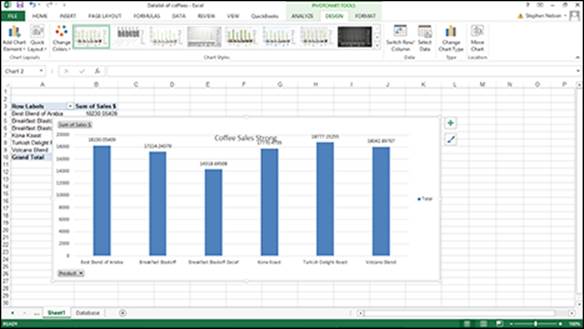
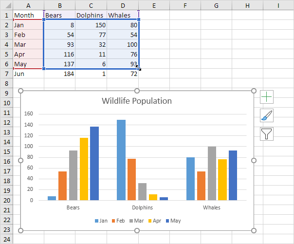
Use pivot chart to create a dynamic chart | WPS Office Academy 2. Then we can see a Chart Elements button on the right side of the PivotChart. 3. Click the button, select the Date Labels option in the popup menu, now the total sales will be displayed above the bar. 4. Then select the Chart Title option to add a title to the pivot chart. Display data point labels outside a pie chart in a paginated report ... Create a pie chart and display the data labels. Open the Properties pane. On the design surface, click on the pie itself to display the Category properties in the Properties pane. Expand the CustomAttributes node. A list of attributes for the pie chart is displayed. Set the PieLabelStyle property to Outside. Set the PieLineColor property to Black. How to Create and Customize a Treemap Chart in Microsoft Excel Simply click that text box and enter a new name. Next, you can select a style, color scheme, or different layout for the treemap. Select the chart and go to the Chart Design tab that displays. Use the variety of tools in the ribbon to customize your treemap. For fill and line styles and colors, effects like shadow and 3-D, or exact size and ... How to update or add new data to an existing Pivot Table in Excel Change the Source Data for your Pivot Table In order to change the source data for your Pivot Table, you can follow these steps: Add your new data to the existing data table. In our case, we'll simply paste the additional rows of data into the existing sales data table. Here's a shot of some of our additional data.

How to Show Percentages in Stacked Column Chart in Excel? Step 2: Select the entire data table. Step 3: To create a column chart in excel for your data table. Go to "Insert" >> "Column or Bar Chart" >> Select Stacked Column Chart . Step 4: Add Data labels to the chart. Goto "Chart Design" >> "Add Chart Element" >> "Data Labels" >> "Center". You can see all your chart data are ... › charts › dynamic-chart-dataCreate Dynamic Chart Data Labels with Slicers - Excel Campus Feb 10, 2016 · You basically need to select a label series, then press the Value from Cells button in the Format Data Labels menu. Then select the range that contains the metrics for that series. Click to Enlarge Repeat this step for each series in the chart. If you are using Excel 2010 or earlier the chart will look like the following when you open the file. Google Data Studio Pivot Tables - Fully Explained In Google Data Studio, click Add a chart and scroll down to select a Pivot table. (The fancy ones can include bar graphs or heat maps.) Voila! A pivot table will appear, pre-populated with what GDS guesses might be some interesting data. This one comes with New Users as the Metric. Excel: How to Apply Multiple Filters to Pivot Table at Once By default, Excel does not allow multiple filters in one field in a pivot table. To change this, we can right click on any cell in the pivot table and then click PivotTable Options: In the new window that appears, click the Totals & Filters tab, then check the box next to Allow multiple filters per field, then click OK: Now if we filter once ...

How To Use Dynamic Data Labels To Create Interactive Excel Charts

Chart.ApplyDataLabels method (Excel) | Microsoft Docs Syntax expression. ApplyDataLabels ( Type, LegendKey, AutoText, HasLeaderLines, ShowSeriesName, ShowCategoryName, ShowValue, ShowPercentage, ShowBubbleSize, Separator) expression A variable that represents a Chart object. Parameters Example This example applies category labels to series one on Chart1. VB Copy Charts ("Chart1").SeriesCollection (1).

Pivot Chart Data Label Help Needed - Microsoft Community

› documents › excelHow to add data labels from different column in an Excel chart? Please do as follows: 1. Right click the data series in the chart, and select Add Data Labels > Add Data Labels from the context menu to add... 2. Right click the data series, and select Format Data Labels from the context menu. 3. In the Format Data Labels pane, under Label Options tab, check the ...

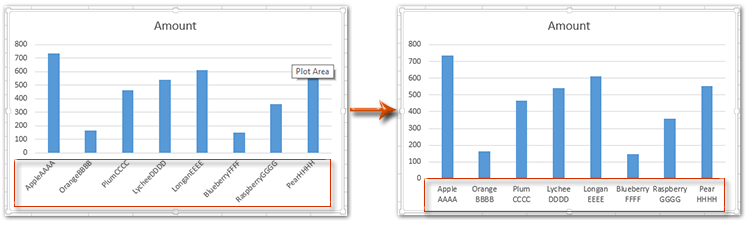
How to wrap X axis labels in a chart in Excel?

answers.microsoft.com › en-us › msofficeFormal ALL data labels in a pivot chart at once - Microsoft ... May 19, 2020 · Hi AaronSchmid ，. I go through the post, as per the article: Change the format of data labels in a chart, you may select only one data labels to format it. However, you may change the location of the data labels all at once, as you can see in screenshot below: I would suggest you vote for or leave your comments in the thread: Format Data ...

image

Dynamic Chart Title by Linking and Reference to Cell in Excel Linking Cell to make Dynamic Chart Title - Step 1: Select a Chart Title. Identify the chart to link a cell reference to the chart title. The following screen-shot will show you example chart title is selected. Dynamic chart title- Cell linking to chart title. Here you can clearly observe that there is no formula is associated to chart title.

How-to Use Data Labels from a Range in an Excel Chart - Excel Dashboard Templates

Tutorial - How to Use a PivotTable to Create Custom Reports in ... 2. Create a pivot table. Select any cell in the source data table, and then go to the Insert tab > Tables group > PivotTable. This will open the Create PivotTable window. Make sure the correct table or range of cells is highlighted in the Table/Range field. Then choose the target location for your Excel pivot table:

Problems formatting pivot chart data labels in Mac v16 - Microsoft Tech Community

python - Adding elements to a chart with Matplot - Stack Overflow Adding elements to a chart with Matplot. pplt.grid (True) pplt.plot (df ['Date'], pivot, label="Pivot") plt.show () I'm drawing a graph with their code. df ['Date'] returns 160 rows of data. the number from the pivot is still equal to. I want to add one more data to this.

How to group (two-level) axis labels in a chart in Excel?

› article › technologyHow to Customize Your Excel Pivot Chart Data Labels - dummies Mar 26, 2016 · Check the box that corresponds to the bit of pivot table or Excel table information that you want to use as the label. For example, if you want to label data markers with a pivot table chart using data series names, select the Series Name check box. If you want to label data markers with a category name, select the Category Name check box.

How to Create Progress Charts (Bar and Circle) in Excel - Automate Excel

Can I add "Count" data label to Pivot Chart showing Averages Can I add "Count" data label to Pivot Chart showing Averages. I have a pivot chart showing data from a recent employee engagement survey. I want to chart the averages, but also provide the "n" for each response as slicers are applied. In the chart below, I'd like the value of the grey column to show as the "n" under the orange column (average ...

Chart's Data Series in Excel - Easy Excel Tutorial

How to Find, Highlight, and Label a Data Point in Excel Scatter Plot? By default, the data labels are the y-coordinates. Step 3: Right-click on any of the data labels. A drop-down appears. Click on the Format Data Labels… option. Step 4: Format Data Labels dialogue box appears. Under the Label Options, check the box Value from Cells . Step 5: Data Label Range dialogue-box appears.

Pivot Chart | ASP.NET Web Forms Pivot and OLAP browser | Syncfusion

How to Add Labels to Scatterplot Points in Excel - Statology Step 3: Add Labels to Points Next, click anywhere on the chart until a green plus (+) sign appears in the top right corner. Then click Data Labels, then click More Options… In the Format Data Labels window that appears on the right of the screen, uncheck the box next to Y Value and check the box next to Value From Cells.

MS Excel 2013: Display the fields in the Values Section in multiple columns in a pivot table

Data Labels in React Chart component - Syncfusion Data Labels in React Chart component 19 Jul 2022 / 8 minutes to read Data label can be added to a chart series by enabling the visibleoption in the dataLabel. By default, the labels will arrange smartly without overlapping. Source Preview index.tsx index.jsx Copied to clipboard

How to Add Total Data Labels to the Excel Stacked Bar Chart – MBA Excel

Add filter option for all your columns in a pivot table Now, I'm trying to figure out how to see the value filter just below the Number filters in the right-click menu, and I dont see in it my Pivot. I have downloaded a sample excel with a pivot which already has the value filter. I'm trying to create my own pivot in this sample excel using the same data set, but I just dont see the value filer.

Working with Multiple Data Series in Excel | Pryor Learning Solutions

support.microsoft.com › en-us › officeAdd or remove data labels in a chart - support.microsoft.com Add data labels to a chart Click the data series or chart. To label one data point, after clicking the series, click that data point. In the upper right corner, next to the chart, click Add Chart Element > Data Labels. To change the location, click the arrow, and choose an option. If you want to ...

Add Total Label On Stacked Bar Chart In Excel - YouTube

Excel Pivot Table tutorial - how to make and use ... - Ablebits 2. Create a pivot table. Select any cell in the source data table, and then go to the Insert tab > Tables group > PivotTable. This will open the Create PivotTable window. Make sure the correct table or range of cells is highlighted in the Table/Range field. Then choose the target location for your Excel pivot table:

Add label to Excel chart line • AuditExcel.co.za

Integrate the WinForms Chart with the Pivot Grid Control Click the Chart Control, click its Smart Tag and select a Pivot Grid instance in the Choose Data Source field. At runtime The following code demonstrates how to use a Pivot Grid as a Chart's data source. C# VB.NET chartControl.DataSource = pivotGridControl; The Pivot Grid control generates all data member names for series generation.

Creating Databound ADF Data Visualization Components

How to Use Excel Pivot Table Label Filters Pivot Table Option Setting To change the Pivot Table option, and allow multiple filters, follow these steps: Right-click a cell in the pivot table, and click PivotTable Options. In the PivotTable Options dialog box, click the Totals & Filters tab In the Filters section, add a check mark to 'Allow multiple filters per field.'

Share :